Experimental Conditions Define the ATP Inference Space

This article illustrates the importance of experimental conditions to evaluate analytical methods. Italicized text is used throughout the article to emphasize key points and illustrate formula variables.
Analytical method validation characteristics accuracy and precision, as defined in ICH Q2,1 are key components in demonstrating the appropriateness of an analytical method. If chosen correctly, a joint metric that considers accuracy and precision criteria together2 ,3 ,4 ,5 will provide a pragmatic criterion for inferences from the analytical method results.
The measurement source used in the assessment against an a priori criterion must be defined carefully. An accuracy or recovery experiment that is part of a method validation exercise, for example, can use measurements of carefully characterized (known) spiked amounts of the active pharmaceutical ingredient (API) in solution to provide an estimate of the measurable amount of the true (spiked) value.4 When measuring API in the drug product (final dosage form), however, there may also be an effect attributed to other components (e.g., excipients) upon complete extraction of the API from product samples.
Without examining representative product samples (in addition to the usual ICH Q2 accuracy validation assessment), the uncertainty of reportable drug product values may not be estimated completely. The interplay between the drug substance, excipients, and drug product manufacturing process can affect the complete drug substance recovery when assaying the dosage form; this can increase the uncertainty of the final result or reportable value.6 If the primary intent is to ensure high quality in the decisions made from the results of drug product samples, then the assessment against a joint accuracy and precision criterion should include evaluation based on experimental units containing drug product (i.e., real) samples.
A staged approach can illustrate the difference in viable inferences between experiments using drug product samples and those that use spiked amounts of API. First, defining an analytical target profile (ATP) can determine the required performance criteria (parameters). Next, method conformance is executed against criteria based on observed data.2 ,4
ATP DEFINED FOR METHOD TRUENESS
In an ICH Q2 validation exercise to assess method accuracy, experimental units can be prepared as spiked API solutions. In addition to typical assessments against individual accuracy and precision criteria, a company may choose to apply an additional criterion for accuracy or trueness by defining an ATP statement such as this one:
ATP1: The procedure must be able to accurately quantify known concentrations of compound name over the range 90%–110% of the nominal concentration with specificity, linearity, accuracy, and precision such that measured concentrations fall within ± 1.0% of the true value with a 95% probability.
This ATP defines the characteristics for the analytical method to be considered acceptable.3 The range (90%–110% of nominal) and the risk (100% – 95% = 5%) of making an incorrect decision concerning both concentration values and (through the 95% probability) the tolerance statement (± 1.0%) is an inherent expression of the true unknown total uncertainty. Because the ATP1 statement attributes constitute unknown parameters, ATP1 should be thought of as a criterion or acceptance domain that defines the maximum decision error of measured concentration values.
Decisions concerning an analytical method acceptance against the ATP1 criterion are based on estimates calculated from real experimental data and serve as an additional internal accuracy validation assessment.
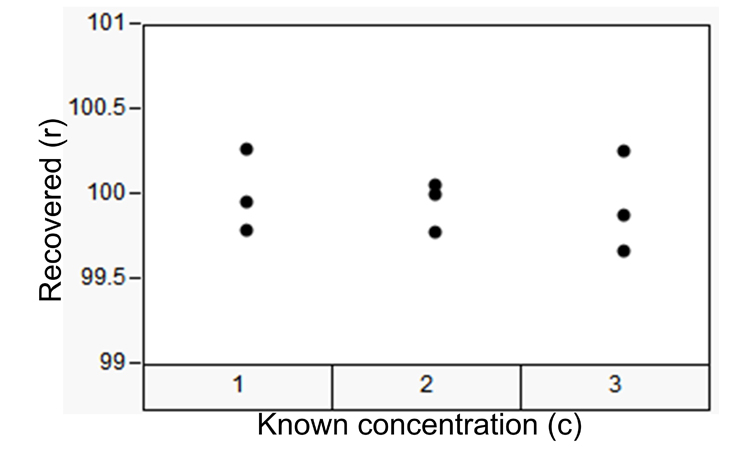
When evaluating the accuracy of an analytical method, spikes of very precisely measured or “known” compound amounts (math TK) are prepared as individual solutions (math TK), usually at three or more concentrations. Figure 1 illustrates such an experimental run. Preparation (math TK) may be an analyte spiked into a mix of product excipients to mimic a typical product sample.7
- 1International Conference on Harmonisation of Technical Requirements for Registration of Pharmaceuticals for Human Use. ICH Harmonized Tripartite Guideline. “Validation of Analytical Procedures: Text and Methodology: Q2(R1).” Geneva: International Conference on Harmonisation. November 2005. http://www.ich.org/fileadmin/Public_Web_Site/ICH_Products/Guidelines/Quality/Q2_R1/Step4/Q2_R1__Guideline.pdf
- 2 a b Martin, Gregory P., et al. “Lifecycle Management of Analytical Procedures: Method Development, Procedure Performance Qualification, and Procedure Performance Verification.” Stimuli to the Revision Process. Pharmacopeial Forum. 39, no. 5 (2013).
- 3 a b Barnett, Kimber, et al. “Analytical Target Profile: Structure and Application throughout the Analytical Lifecycle.” Stimuli to the Revision Process. Pharmacopeial Forum 42, no. 5 (January 2016). https://www.researchgate.net/publication/308467600_Analytical_target_profile_Structure_and_application_throughout_the_analytical_lifecycle
- 4 a b c Hubert, P., et al. “Harmonization of Strategies for the Validation of Quantitative Analytical Procedures. A SFSTP Proposal—Part I.” Journal of Pharmaceutical and Biomedical Analysis 36 (2004): 579–586.
- 5Barnett, K.L., B. Harrington, T. W. Graul. “Validation of Liquid Chromatographic Methods.” In Liquid Chromatography, edited by S. Fanali, P. R. Haddad, and C. F. Poole. Waltham, MA: Elsevier, 2013.
- 6US Pharmacopeia and National Formulary. USP 39–NF 34, Supplement 2, General Notices and Requirements. 2016.
- 7Ermer, J., and C. Agut. “Precision of the Reportable Result: Simultaneous Optimization of Number of Preparations and Injections for Sample and Reference Standard in Quantitative Liquid Chromatography. Journal of Chromatography (1 August 2014).
While other experimental factors may also be examined in the accuracy experiment (e.g., series, instruments, analysts) and their contributions to the total variability examined, the inference is on the accuracy (trueness) of the method, as the reported measurement consists of well characterized (known) concentrations and not real-life samples of the drug product.
As an example of qualifying an analytical method against the a priori– defined ATP criterion, consider the following accuracy validation experiment, which consists of three spiked amounts of well characterized (known) content, with concentrations increasing from level 1 to level 3.
Values in Table A show the recovered amount of known quantities of analyte dissolved in diluent and assayed for content. The three concentration levels represent different amounts of the dissolved known ingredient. Thus, the experimental variability from concentration to concentration represents variation among standard preparations with differing levels of analyte concentration. Variability within concentration levels represents the contribution of variability attributed to weighing the analyte and pipetting the known concentrations, as well as contributions from the separation, detection, and data analysis. We can assess this data set against the criterion defined in ATP1 to say something about the method trueness or accuracy. Table B shows the sums of squares (derived from the data in Table A) required to estimate the random effects of the precision components.
| Known* Concentration | % Recovered |
|---|---|
| 1 | 99.95 |
| 1 | 100.27 |
| 1 | 99.79 |
| 2 | 99.78 |
| 2 | 100.00 |
| 2 | 100.05 |
| 3 | 99.67 |
| 3 | 99.88 |
| 3 | 100.25 |
| * While the true content is never really “known,” the exactness of API powder weighing and acquiescing affords an extremely precise estimate of the true content. |
|

| Source | Concentrations | Preparations | Total (corrected) |
|---|---|---|---|
| df | \( \left( c-1 \right) =2 \) | \(c \left( r-1 \right) =6 \) | \( \left( cr-1 \right) =8 \) |
| Sums of squares (SS) | \( \sum _{i=1}^{c} \left( y_{i}-y \right) ^{2}= 0.0085 \) | \( \sum _{i=1}^{c} \sum _{j=1}^{r} \left( y_{ij}-y_{i} \right) ^{2}=0.3321 \) | \( \sum _{i=1}^{c} \sum _{j=1}^{r} \left( y_{ij}-y \right) ^{2}=0.3406 \) |
| Mean squares (MS) | \( \frac{SS_{concentrations}}{c-1}=0.0043 \) | \( \frac{SS_{preps}}{c \left( r-1 \right) }=0.0553 \) | |
| Expected mean squares | \( \sigma ^{2}+3 \sigma ^{2} \) | \( \sigma ^{2} \) |
The precision is then calculated as:
$$ \begin{align} \sigma_{IP} & = \sqrt{ \frac{1}{r} \times MS_{concentrations} + ( 1 - \frac{1}{r} ) \times MS_{preps}} \\ \sigma_{IP} & = \sqrt{ \frac{1}{3} \times 0.0043 + ( 1-\frac{1}{3} ) \times 0.0553} \\ \sigma_{IP} & = 0.196 \end{align} $$
The accuracy (math TK = 99.93) and precision (math TK = 0.196) estimates may now be used to assess method performance against the ATP1 criterion. Confidence in this assessment may be achieved by several techniques. Using experimental data, two statistical procedures provide confidence of meeting the a priori ATP1 criterion: the gamma-content tolerance interval,3 ,8 and the large-sample joint confidence interval.9 The upper 100(1 - math TK)% confidence bound can also provide confidence of achieving the ATP1 criterion. This upper bound [math TK] is presented by Graybill and Wang.3 ,8 The formula is:
$$ U_{GW}= \sigma _{IP}+ \sqrt{H_{1}^{2} ( \frac{1}{r} ) ^{2}MS_{conditions}^{2}+ H_{2}^{2} ( 1-\frac{1}{r} ) ^{2}MS_{samples}^{2}} $$
where
$$\begin{align} H_{1} & = \frac{c-1}{ \chi _{ \alpha , c-1}^{2}}-1 \\ H_{2} & = \frac{c ( r-1 ) }{ \chi _{ \alpha , c ( r-1 ) }^{2}}-1 \end{align} $$
and \( x^2_{a,df} \) is the \(a \)th quantile of the cumulative x2 distribution with dfdegrees of freedom.
For this example, UGW= 0.298, the two-sided y tolerance interval for is:3 ,8
$$ \bar y \pm Z_{\frac{1- \gamma }{2}}\sqrt{ ( 1+ \frac{S_{1}^{2}}{rc {\sigma_{IP}}^2} ) \times U_{GW}} $$
where Z(1-y)/2 represents the 100(1 - y)/2% quantile of the standard normal.
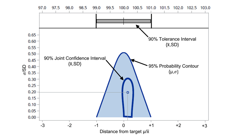
Similarly, a joint y confidence interval for the mean and variance may be used to demonstrate acceptability.9 Graphically, this joint confidence interval is an ellipse centered at (\( \bar y, \sigma_{IP}\)) of the (x,y)coordinates in the ATP graph.
The equations for this joint confidence interval are:
$$\begin{align} x & = \bar y + \sigma _{IP}\sqrt{2\frac{F_{2, n-2, 1- \alpha }}{n}} \times cos ( t ) \\ y & = \sigma _{IP}+ \sigma _{IP}\sqrt{4\frac{F_{2, n-2, 1- \alpha }}{n}} \times sin ( t ) \end{align} $$
where t ranges from 0 to 2_pie radians, and F2,n-2,1-a represents the 100(1 - a)% quantile of the F distribution (Figure 2).
- 3 a b c
- 8 a b c US Pharmacopiea. PF Online. In-Process Revision: <1210>. Statistical Tools for Procedure Validation. Pharmacopeial Forum 40, no. 5 (2014).
- 9 a b De los Santos, P., L. Pfahler, K. Vukovinsky, J. Liu, and B. Harrington. “Performance Characteristics and Alternative Approaches for the ASTM E2709/2810 (CUDAL) Method for Ensuring that a Product Meets USP <905> Uniformity of Dosage Units.” Pharmaceutical Engineering (October 2015): 44-56.

Indeterminate of the confidence interval applied, both the joint confidence interval (ellipse) and the tolerance interval (rectangle) illustrate acceptance against the a priori–defined ATP1 criterion.
Based on observed data, an interval allows for a statement of confidence (90% in the example) concerning ATP1 acceptance. In this example, the method may be judged as accurate, since data show that the method can provide a measured amount of a well-characterized concentration within ±1% with at least 95% probability. Confidence in this statement, based on data generated by the experiment, is 90%.
While this example illustrates an experiment that applied an analytical method to a known drug substance, it is equally applicable to a synthetic mixture of the known drug substance and drug product excipients. In either case, a drug substance or drug product accuracy experiment, the accuracy of the method can be determined.
ATP Defined for Reportable Drug Product Assays
When evaluating an analytical method to report drug product results, sample preparation includes not only the API and drug product excipients, but the dosage form itself. Therefore, any assessment used to infer method ability to elicit decisions concerning drug product reportable values should include the drug product sample. This differs from the validation exercise of assessing method accuracy as illustrated above.
The following is a hypothetical ATP statement, defined a priori to any experimental data analyses, for judging reportable assay values for a drug product.2 ,5
Drug product sample preparation includes not only the API and drug product excipients, but the dosage form itself
ATP2: The procedure must be able to accurately quantify compound name in dosage form over the range 90%–110% of the nominal concentration with accuracy and precision such that reportable assay values fall within ± 3.0% of the true value with at least 95% probability.
Like ATP1, ATP2 defines the characteristics by which the analytical method will be considered acceptable.3 The distinction is that ATP2 provides an a priori criterion to judge dosage form samples (drug product assay values) that incorporate the dosage unit sample preparation technique. Because the ATP2 statement attributes constitute unknown parameters, ATP2 should be considered a criterion or acceptance domain. ATP2 defines the maximum decision error of reportable assay values involved in lot release against specifications, stability trending assessments, and experimental outcomes in formulation or process development exercises of a finished drug product lot. Decisions concerning an analytical method acceptance against the ATP2 criterion are based on sample estimates calculated from real experimental data.
To enable inferences on reportable values,3 the precision estimate must consist of components inherent in the drug product sample and the method applied to it. Variability of the reportable drug product potency value is contributed by both the method and dosage-unit variability.7 ,10 Other factors that may also contribute to the total variability can be assessed in an intermediate precision study, ultimately evaluating the method against the criterion defined in ATP2.
Figure 3 illustrates the sample replication component of this type of experiment. The variability of such an assay consists of the contribution of differences of the average of r product sample preparations (S), each comprising k dosage units (du).10
By replicating Figure 1 for any number of ICH Q2–defined intermediate precision components (e.g., series, instruments, analysts), estimates of these components can be partitioned from the total experiment variability along with the above assay method repeatability component to determine their contributions to total analytical variability.
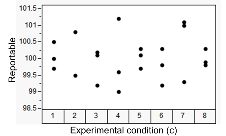
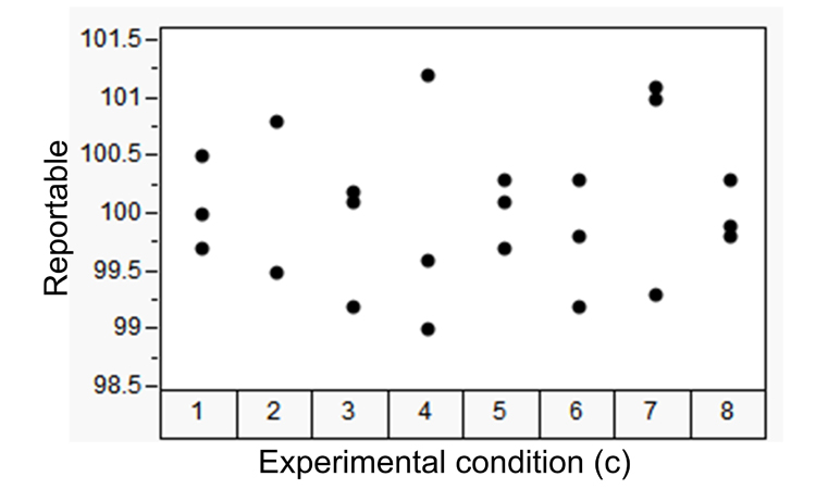
Consider the experimental data shown in Table C, consisting of eight independent experimental conditions [combinations of analysts and instruments, (c)]; each with three product sample replicates (r). The values in Table C are the average of five dosage units dissolved in media and assayed for content. The eight experimental conditions represent different analyst and instrument combinations. Variability from condition to condition reflects variation among analyst and instrument combinations (an intermediate precision component). Variability within conditions represents variation from sample to sample. We can assess this data against the criterion defined in ATP2 to determine the method’s ability to elicit risk-based decisions concerning reportable values (sample assays). This is achieved by estimating the overall average and the composition of the precision components.7 , 10
| Experimental Condition |
Sample Number | ||
|---|---|---|---|
| 1 | 2 | 3 | |
| 1 | 99.7 | 100.5 | 100.0 |
| 2 | 99.5 | 100.8 | 99.5 |
| 3 | 100.1 | 99.2 | 100.2 |
| 4 | 101.2 | 99.6 | 99.0 |
| 5 | 100.3 | 100.1 | 99.7 |
| 6 | 99.2 | 100.3 | 99.8 |
| 7 | 101.0 | 101.1 | 99.3 |
| 8 | 99.9 | 100.3 | 99.8 |

Table D shows the sums of squares derived from the data in Table C required to estimate the random effects of the precision components.
| Source | Concentrations | Preparations | Total (corrected) |
|---|---|---|---|
| df | \( \left( c-1 \right) =7 \) | \( c \left( r-1 \right) =16 \) | \( \left( cr-1 \right) =23 \) |
| Sums of squares (SS) | \( \sum _{i=1}^{c} \left( y_{i}-y \right) ^{2}= 0.894 \) | \( \sum _{i=1}^{c} \sum _{j=1}^{r} \left( y_{ij}-y_{i} \right) ^{2}=7.45 \) | \( \sum _{i=1}^{c} \sum _{j=1}^{r} \left( y_{ij}-y \right) ^{2}=8.34 \) |
| Mean squares (MS) | \( \frac{SS_{concentrations}}{c-1}=0.128 \) | \( \frac{SS_{preps}}{c \left( r-1 \right) }=0.466 \) | |
| Expected mean squares | \( \sigma ^{2}+3 \sigma ^{2} \) | \( \sigma ^{2} \) |
The intermediate precision is then calculated from the random effect estimates:
$$\begin{align} \sigma _{IP} & = \sqrt{\frac{1}{r} \times MS_{condition}+ ( 1-\frac{1}{r} ) \times MS_{samples}} \\ \sigma _{IP} & = \sqrt{\frac{1}{3} \times 0.128+ ( 1-\frac{1}{3} ) \times 0.466} \\ \sigma _{IP} & = 0.6 \end{align} $$
As in the first example, confidence in the analytical method’s ability to produce results that adhere to the decision rule of the ATP may be calculated from experimental data.
The graph in Figure 4 illustrates the ß-content tolerance interval3 ,8 and the joint y confidence interval9 methods using 90% confidence as the experimental guarantee. Including the tolerance interval within the ATP2 bounds (±3 of target) and the joint data confidence ellipse within the ATP2 probability contour parabola (shaded area in Figure 4) indicate at least 90% confidence of meeting the ATP2 criterion. Figure 4 also shows the average (\( \bar x\)) and standard deviation (SD) of multiple drug product samples. Since the true sample average is never known, \( \bar x\) inferences must incorporate knowledge gained from separate extraction studies to account for systematic method bias. Figure 4 illustrates this adjustment for an accuracy recovery estimate of –0.4% observed in a previous accuracy validation experimental exercise.

As in the previous example, the joint confidence interval (ellipse) and tolerance interval (rectangle) illustrate acceptance against the a priori–defined ATP2 criterion. This implies that a statement of confidence (90% in the example) concerning ATP2 acceptance for this method can now be made. That is, the method is capable of providing reportable values within ±3% label claim of the true, unknown sample value with at least 95% likelihood. Based on the data in this experiment, the confidence level is 90%. Of particular note is the proclamation concerning reportable drug product values, because the experiment was executed utilizing drug product samples, not a synthetic mixture.
While the statistical assessments in Figure 2 and Figure 4 are similar, the inference space changes. In the second example, the dosage unit variability estimates (Figure 4) reflect the contribution of the drug product sample variability to the reported potency assay variability. This indicates that evaluation against the ATP2 criterion helps infer risk-based decisions on the reported drug product assay value by assigning a risk threshold (probability) that the reported value will exceed a maximum distance from the true, unknown assay of the sample.
Experimental conditions are critical for determining which inferences can be made
Conversely, the accuracy validation experiment (Figure 1) provides an estimate of variability about known spike amounts (math TK) that measure variability about analyte weighing and pipetting of known concentrations. Evaluating the ATP1 criterion speaks to the inherent trueness (bias) of the method by assigning a risk of how much known standard concentrations may differ.
This distinction is necessary to ensure appropriate inferences concerning the measured results. The qualifying difference is the experimental conditions: By using known concentrations—as illustrated in the first example (ATP1)—the inference is to a measurement of accuracy or trueness, an ICH Q2 validation exercise to estimate method bias. This is an extremely useful exercise as the assessment of known concentrations provides the best estimate of method trueness or accuracy. While the accuracy assessment is critical to the method validation exercise, this experiment says little about the risk of inferences concerning a drug product reportable result value.3 It is equally important to assess reportable value variability as well via an experiment consisting of variance components of drug product samples, as illustrated in the second example.
Conclusion
The experimental conditions under which results will be generated are critical for determining which inferences can be made. Assessing measurements from known concentrations against an a priori–defined criterion (ATP) provides an additional validation assessment of the accuracy attribute defined in ICH Q2. For drug product assays in particular, evaluating drug product samples against an a priori ATP statement provides a pragmatic means for assessing the confidence (guarantee) that the analytical method will elicit reportable values capable of meeting a pragmatic decision rule—e.g., reportable values will remain with ±3% label claim of the true, unknown sample value.
Acknowledgments
The authors thank two anonymous reviewers whose comments provided greater clarity to the text and the following for their insightful discussions from which this manuscript was inspired: Beverly Nickerson, Loren Wrisley, and Kim Vukovinsky.


